Category: R/V Kilo Moana Page 1 of 5

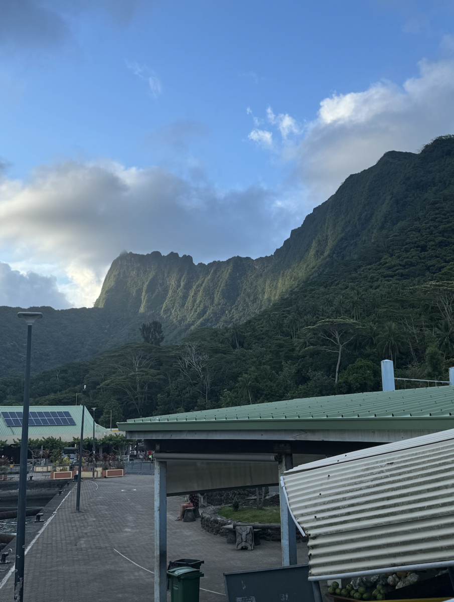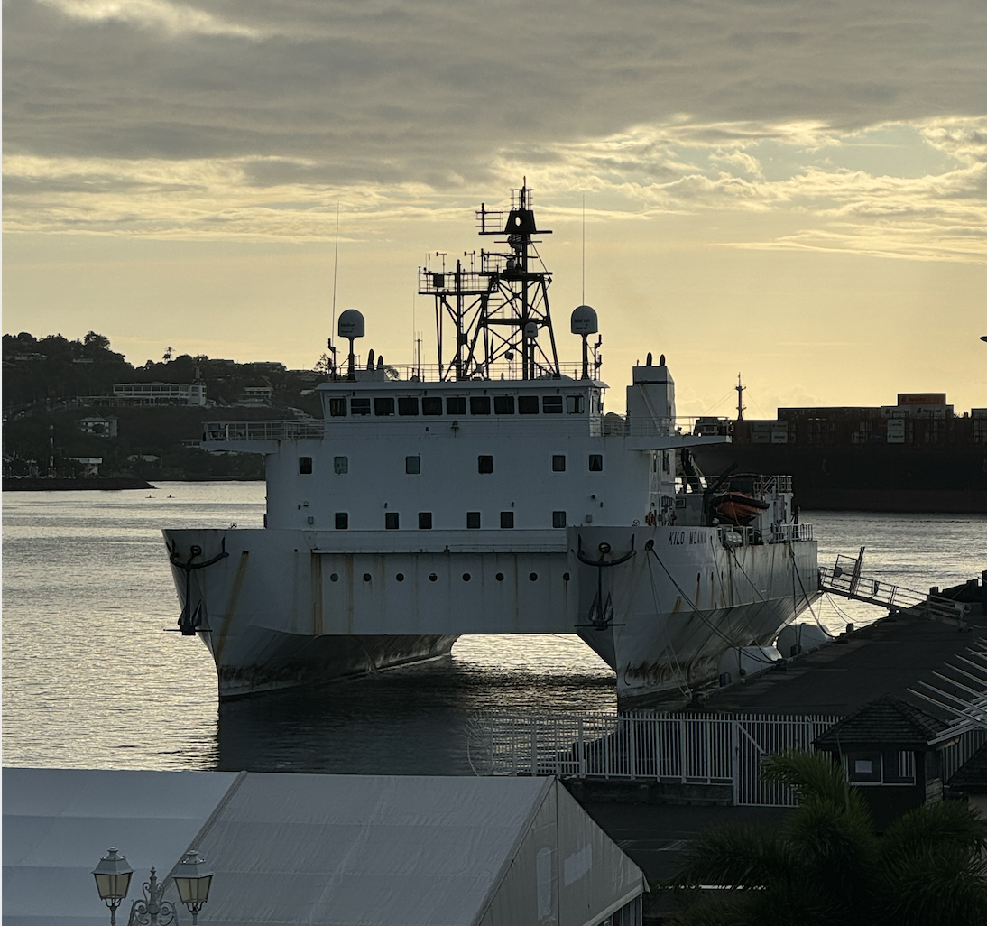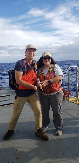
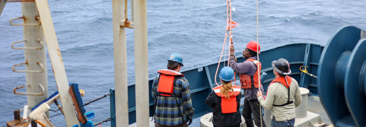
On Monday we took an official tour of all the spaces in the CMORE building associated with the HOT team. We had been introduced to the spaces we were using so far but it was cool to see the full picture!

Unfortunately due to an allergic reaction I was out for part of Monday and Tuesday, but by Wednesday I was feeling ready to jump back in!

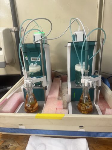
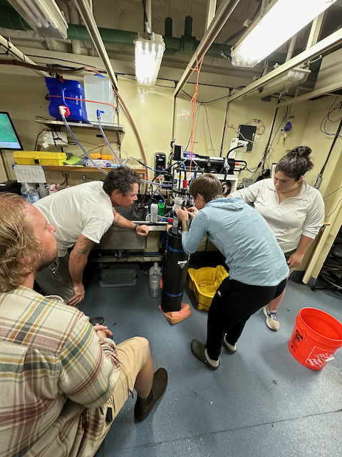
On Wednesday I learned how the HOT team determines the total dissolved inorganic carbon (DIC) in seawater samples. They use a machine called a Single Operator Multi-parameter Metabolic
Analyzer, or SOMMA. Dan Sadler walked us through each step that the SOMMA uses, and I practiced running samples.

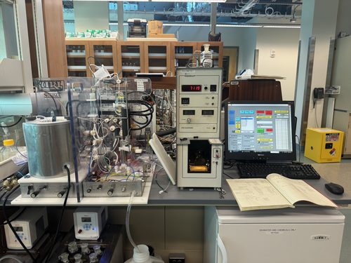
First, water samples are placed in a water bath to achieve a constant temperature. A second water bath surrounds the sample when it is connected to the SOMMA for processing. The SOMMA begins the analysis process by rinsing the interior plumbing twice with sample, then pumps a set volume of sample into a secondary flask, also surrounded by a water bath. The SOMMA uses an open circuit and the conductivity of seawater to determine when each chamber is sufficiently filled.

The set volume of sample then moves on to the ‘stripping chamber’, where it is reacted with phosphoric acid. This change in pH shifts the chemical equilibrium so that all DIC in the sample is in the form of CO2. In the same chamber in the SOMMA, carbon dioxide free air bubbles through a frit to carry CO2 derived from the sample on to the next processing step without any seawater or acid.

The CO2 derived from the sample moves through a condenser that removes water vapor by chilling the sample, then passing it through a column of magnesium perchlorate. Then, the gas moves on to the coulometer cell.

In the coulometer cell, the CO2 derived from the sample is returned to solution by reacting with an absorbent containing ethanolamine. As CO2 enters the coulometer cell, it acidifies the solution( producing H+), causing a blue indicator dye to fade to clear. A beam of light passes through the solution, and when the transmission of light begins to increase, the machine understands that CO2 is being added and starts to titrate.

The machine titrates by adding a measurable number of electrons to the coulometer cell. An electric current is applied to a silver anode submerged in an anode solution, attached as an ‘arm’ alongside the larger cathode chamber of the coulometer cell where the sample is deposited. The anode and cathode chambers are separated by a frit that allows electrons to pass through, so when more electrons are added to the anode chamber, the concentrations balance and more electrons are added to the cathode chamber as well. When the SOMMA detects CO2 in the coulometer cell and starts to titrate, it keeps a ‘count’ that directly corresponds to the number of electrons added, based on the time interval, current and voltage.

When electrons move into the cathode chamber, they react with water, producing hydrogen (H2) and hydroxide (OH-), a base that neutralizes the H+ created by introducing CO2 from the sample. This neutralization is reflected by the indicator dye, which becomes darker in color. When the transmission of light drops to 29%, the machine stops adding electrons and waits. The SOMMA records counts every minute, but since CO2 continuously moves into the coulometer during the analysis process, it doesn’t stop titrating until the count is below baseline for four consecutive minutes. When the count is at or below baseline, this means that no more CO2 is being introduced to the sample because all of the CO2 has already been ‘used up’, neutralized, and accounted for.

Finally, we can account for the number of counts included in the background rate (about 5 counts for minute with the HOT team’s current SOMMA) by multiplying the background rate by the time required for analysis, which can vary for each sample. Then, we can subtract this from the total counts and calculate the corresponding number of electrons needed to neutralize all of the CO2. Since the ratio of H+ to OH- is one to one, this also tells us the moles of CO2 present in each sample.

We already know that the SOMMA uses a fixed volume at a specific temperature, so with the moles of CO2 in the final step we can calculate the concentration of DIC per kilogram of seawater.

All of these reactions happen internally within the SOMMA, and proceed automatically after inserting the sample and starting the analysis process on the associated computer. It’s an incredible instrument and I was so excited to learn how it works!

The SOMMA only uses a small portion of each water sample for its analysis: so the remaining water is titrated to determine alkalinity. The HOT team collects enough water to redo either the SOMMA analysis or the alkalinity titration, in case any problems arise during analysis.

In the afternoon, I met with Dr. Fanny Girard, a professor studying deep sea corals. My undergraduate research focused on habitat mapping at a methane seep, and I’m also interested in deep sea ecology, so I was excited to talk in person! She was able to help me identify the family of some black corals that I had observed at my study site (Pythia’s Oasis) and show me some beautiful corals of her own from her latest cruise.

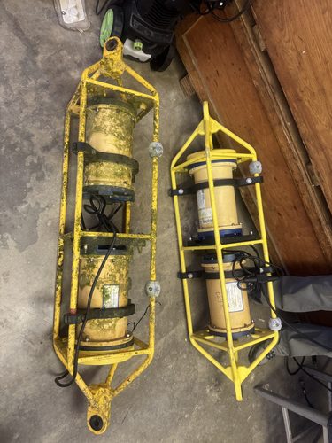
On Thursday, we went to work with Dan Fitzgerald and saw his lab at the Marine Sciences Building. He had recently returned from a WHOTS cruise where a mooring was recovered, so he had some ADCPs and mini-CATs with new data to download! ADCPs, or acoustic doppler profilers, measure current speed throughout the water column by interpreting the reflectance of acoustic pings off of particles moving with the water.

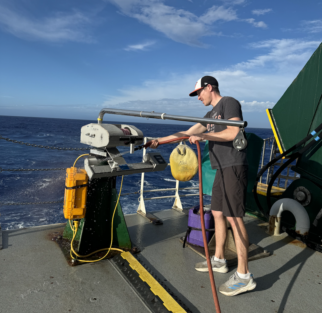
Mini-CATS measure conductivity (salinity) and temperature. We pressure washed the instruments to clean off biofouling before carrying them up to the office.

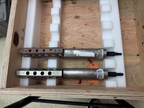
Dan uses a variety of cables to establish direct communication with each instrument, run commands, and download data, depending on the generation of each instrument. He gave us an introduction to serial communications and gave us some tips on navigating and troubleshooting. I got to ask lots of questions about ADCPs and take them apart to access the data! We learned that mooring ADCPs have additional considerations compared to shipboard ADCPs, since you can’t use a ship’s heading, and moorings can spin and tilt in the current. Instead, WHOTS ADCPs have a magnetic compass and tilt sensors. The magnetic fields around the battery packs, which are created in-house, can interfere with the compass – so Dan taught us that it’s important to degauss our instruments.

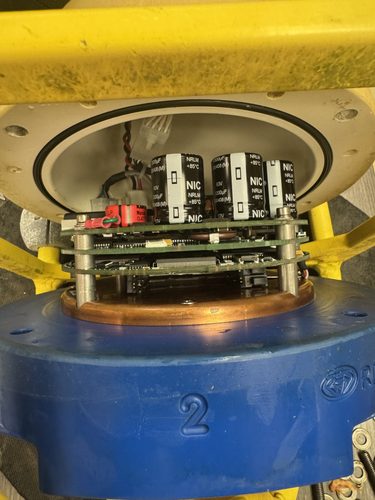
That afternoon, I had the chance to meet with Dr. Julia M. Hummon and Dr. Eric Firing, who lead shipboard ADCP management in the UNOLS fleet and beyond. They reach out to ships if they notice problems with any of their ADCPs, guide troubleshooting, and oversee installation, as well as leading workshops and processing ADCP data for their clients. They had some great insights about the skills and qualities necessary to be successful in their field.

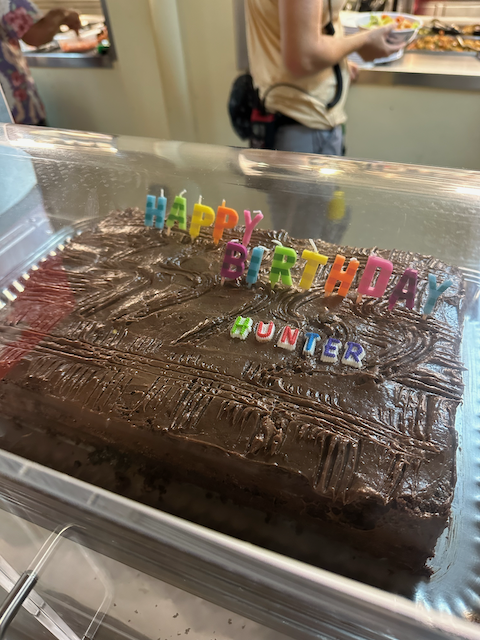
On Friday, I traveled back down to the beach lab to work with Hunter Adams, a SUBSEAS technician. The SUBSEAS program focuses on understanding the cycling of organic carbon between the surface ocean and the mesopelagic. This program works closely with the HOT team and will be joining us on our next cruise!

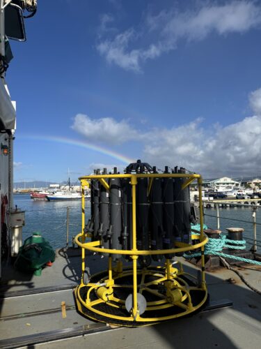
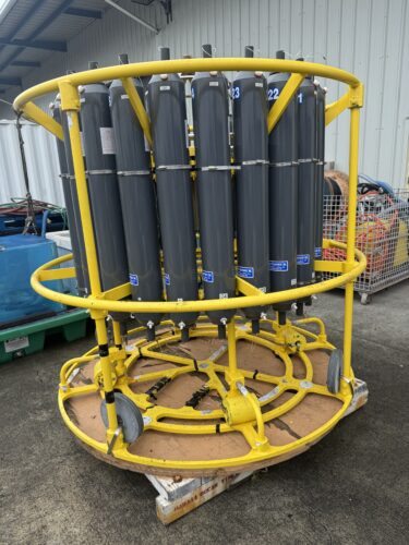
While working with Hunter we learned how to replace hardware on a trace metal CTD rosette, and got an introduction to some of SUBSEAS’ other instruments.

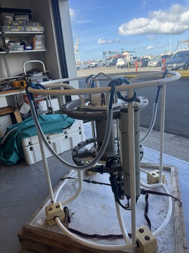
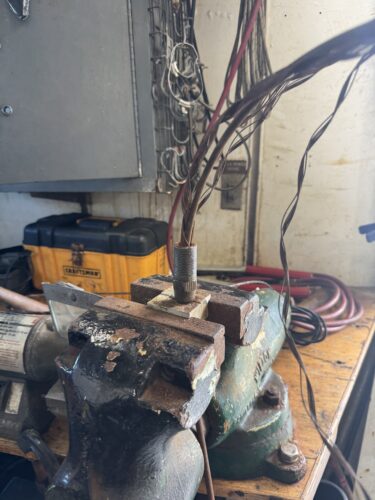
We saw the WireWalker, a profiler that uses wave energy to ‘climb’ down its own tether to record data across the water column, and Hunter demonstrated how to talk to the instrument using serial communications. He gave us some advice for troubleshooting and walked us through testing the connection for each pin on a cable when interfacing between multiple instruments. WireWalker uses a CTD logger in combination with other instruments, so proper communication and programming is especially important for this profiler.

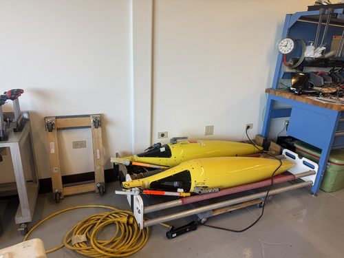
Though SUBSEAS’ Seaglider was all boxed up, there were some other Seagliders in the lab! Hunter talked us through their basic mechanics and deployment process. SUBSEAS’ Seagliders have a CTD, fluorometer, dissolved oxygen, and a fragile shear sensor that makes deployment and recovery a delicate operation!

Finally, we bench tested a Vertical Microstructure Profiler, an instrument that measures small differences in shear. We blocked off the instrument in a faraday cage of tinfoil connected to ground, turned off the lights, and avoided moving around the room while the instrument ran. The sensors operated as expected once we had blocked out background electrical noise, so they should be ready to go for their next use case.

All in all, I had an amazing week continuing to learn and meet new people!

Week 2: Emily Pinneo

By Emily Pinneo

On October 17, 2026

In R/V Kilo Moana, University of Hawaiʻi at Mānoa, SOEST

We embarked on HOT Cruise 367 early Sunday morning. After a little time to unpack, we completed our safety drills and left the harbor.

We practiced sampling a CTD for oxygen, chlorophyll, and nutrients on our first cast, and recorded the surface temperature with a thermometer over the side. We also shadowed a HOT technician while they prepared and analyzed pH samples from the CTD. Each sample was placed into a specialized container with a set amount of pH indicator dye, and run through a spectrophotometer. In order to ensure accuracy, the pH of the dye was tested and adjusted before use, and samples were kept at a constant temperature using a water bath.

Next, we got started preparing sediment traps for deployment. The first step was preparing the ‘HOT sauce’: a mixture of formalin, seawater, and salt to fix sediment samples and keep them in place. After filling each sediment trap, we deployed them over the side on a cross.

Finally, we learned how to record meteorological observations. Every four hours, we recorded latitude, longitude, atmospheric pressure, and humidity. We measured the humidity manually using a psychrometer on the ship’s bow.

After my shift, I had the chance to go star gazing, and saw beautiful views of the Milky Way!

On Monday, we focused on sampling our CTD for particulates, including carbon, nitrogen and phosphate (BPO4).

For particulate carbon and nitrogen, we collected large carboys of water from each CTD bottle, then filtered each carboy using positive pressure (nitrogen gas). Some carboys took longer to filter than others – another HOT technician noted that certain depth ranges (~175 m) had more material in the water and clogged up the filters more quickly. Once each carboy finished filtering, we collected the filters for further processing. Back on shore, each filter will be combusted – thermal conductivity sensors can be used to determine the composition of carbon and nitrogen present on each filter. The filters themselves are made of glass microfiber and will not burn – in fact, they are combusted before use as well, in order to remove any contamination.

The process of collecting particulate phosphate (BPO4) samples was similar to collecting particulate carbon and nitrogen – large carboys were filled with water and filtered. However, the preparation and analysis is conducted differently. BPO4 filters are acid cleaned as well as combusted before use. After BPO4 found on the filters is combusted and converted into orthophosphates, they are dissolved in various acids to create a colored solution that is then measured with a spectrophotometer.

On Tuesday, we learned how to sample for ATP – a useful method to estimate microbial biomass (excluding viruses). First, we filtered the seawater from our CTD using negative pressure (a vacuum pump). This step captured ATP associated with living biomass but not ATP dissolved in the water, which passed through the filter. Next, each filter was boiled in a test tube containing Tris-buffer, to extract the ATP, before being frozen to preserve each sample for further analysis.

ATP samples are analyzed using the firefly bioluminescence assay, where the enzyme luciferase (found in fireflies) catalyzes the oxidation of ATP dependent D-luciferin to oxyluciferin, and emits light. The amount of light emitted is proportional to the number of enzymes activated, which is in turn proportional to the available quantity of ATP in each sample. By measuring the amount of light generated with a luminometer, we can measure how much ATP is present. I was super excited to learn about this method, which was new to me!

Next, I learned how to fix and flash freeze samples for microbial analysis. First, we added a low concentration of formaldehyde, and then we dipped each sample tube into a dewar of liquid nitrogen.

We continued taking samples from our CTD water. We sampled for chlorophyll, by filtering seawater and placing filters in test tubes with acetone to extract pigment. We were careful to wrap each chlorophyll sample with tinfoil to prevent the pigments from degrading with exposure to light. We collected water to test for salinity in order to ground-proof the conductivity sensors on the CTD.

I also shadowed a marine engineer while he collected zooplankton samples, and observed the plankton under the microscope.

Finally, we deployed our CTD on a deep cast to 4725 meters, and sent along a bag of Styrofoam cups! When we recovered the CTD, the Styrofoam cups had all shrunk in size due to the pressure at depth.

On Wednesday, I was trained on conducting Winkler titrations to determine the quantity of dissolved oxygen in a water sample. After my training, I worked on running titrations for the rest of my shift. I was excited to practice some chemistry!

On Thursday, I took a tour of the engine rooms belowdecks and finished up the rest of the oxygen titrations. I also spent some time familiarizing myself with the various instruments and data streams coming through the computer monitors in the CTD lab, including the ADCP. Near the end of my shift, a storm petrel flew into the loading bay and had to be relocated!

On Friday, we returned back to port in Honolulu. After packing up and cleaning our rooms, we unloaded all of our cruise gear and samples, and put them away back in the lab.

I loved spending time at sea, and I can’t believe my first cruise with the HOT team is already over! I learned so much about different instruments and sampling techniques, and I can’t wait to continue my work over the next couple of weeks.

The weather was beautiful as we unloaded and we had a little bit of a rain shower. Apparently, the real treasure at the end of the rainbow is a CTD!

Week 1: Emily Pinneo

By Emily Pinneo

On October 10, 2026

In R/V Kilo Moana, University of Hawaiʻi at Mānoa, SOEST

I arrived in Honolulu this Tuesday and had the chance to meet the team and assist with mobilization for our upcoming cruise. It was amazing getting to see and participate in the work that goes into maintaining such a high-quality time series dataset!

On Wednesday, I completed a safety training quiz and assisted the HOT team at their onshore labs in the C-MORE Hale building on campus. I helped prepare water for nitrogen fixation incubation experiments, which was a lot of fun – after the team removed other gasses from the seawater, we chilled the water and enriched it with nitrogen. In order to dissolve the nitrogen bubbles into the water, we used a highly technical tool – a flyswatter!

Next, I helped out with acid cleaning to remove any trace metal contamination from some of the HOT team’s lab equipment. In between tasks, I could look out the window and see White Fairy Terns, or Manu o Kū, perching in the nearby trees. The team was very welcoming and showed me a good cafe to eat at for lunch, with amazing banh mi!

After that, I learned how to run chloropyll samples with the HOT team’s fluorometer. The team had conducted an extra transect between their normal station and shore, and still had samples left over, so I was able to practice. At first the fluorometer was acting up, but the readings returned to normal after we turned it off and back on again!

After work, I was able to explore the campus Japanese gardens near my lodging.

On Thursday, I toured the ‘beach lab’ at the marine operations center and got started preparing a CTD for the cruise. We got to see different winches, sediment traps, wave buoys, and the ROV Lu’ukai, as well as getting our first glimpse of the R/V Kilo Moana!

We learned how to string the niskin bottles on a CTD rosette – which, like a lot of things, is easier with a little teamwork! I had cocked CTD bottles before, but I had never previously worked with the internal springs that hold the caps in place. This experience gave me a much better understanding of how these instruments work – the top and bottom caps of each niskin bottle have to be connected with the right length of cable and spring, without damaging the O-rings that help the bottles seal shut after sampling. The HOT science team re-strings their CTD bottles before each cruise to avoid leaving them under tension and reduce unnecessary wear and tear on their equipment.

Next, we were introduced to the sensor array on the CTD itself. The CTD had hit the seafloor during a cast on a previous cruise, so they wanted to replace the more susceptible sensors in case of any damage. One of our mentors demonstrated how to replace a conductivity sensor, and then gave us a chance to practice. Then, we learned how to update the calibration files needed for the new sensors. The HOT team uses two duplicate temperature, conductivity, and oxygen sensors on each CTD to ensure consistent measurements, and updates calibrations after each cast by ground-proofing each measurement with lab analyses on water samples.

On Friday, we mobilized for our first cruise! The team worked seamlessly to get three vans full of equipment onto the ship and set up in the lab, including positive and negative pressure pumps for filtration. Next, we shadowed our mentor while he completed a CTD cable termination – a process we’ll be able to practice later in the internship. Then, the team tested the termination under tension using a crane on deck. For lunch, we stopped by a local fish market with amazing poke bowls!

All in all, I’m amazed by how much I’ve learned in just three days and I can’t wait for our upcoming cruise!

Intro: Emily Pinneo

By Emily Pinneo

On October 2, 2026

In R/V Kilo Moana, University of Hawaiʻi at Mānoa, SOEST

Hello! My name is Emily, and I am excited to join the Hawaii Ocean Time-series team as a UNOLS MATE intern this fall. I will be participating in cruises KM26-13 HOT 5 and KM26-14 HOT 6 on the R/V Kilo Moana.

I studied Oceanography at the University of Washington, where I discovered a love for marine technology and fieldwork. I worked for the Ocean Observatories Initiative Regional Cabled Array while in school, where I helped maintain an array of deep sea instruments and participated in two research cruises on the R/V Thomas Thompson and R/V Atlantis. I am interested in deep sea ecology and conservation, and also completed an undergraduate thesis project mapping the benthic fauna at the methane seep Pythia’s Oasis. I can’t wait to broaden my technical and lab skills with this new internship opportunity!

I love incorporating marine science into art, including drawing, painting and pottery. In my free time, I also enjoy reading, creative writing, and gardening. I’m excited to travel to Hawaii and meet the team!

Intro: Drake goes to Hawai’i

By Drake Lee-Patterson

On September 24, 2026

In R/V Kilo Moana, University of Hawaiʻi at Mānoa, SOEST

Hello all!

My name is Drake, and I’m very excited to be joining the Hawai’i Ocean Time-series for their upcoming projects KM26-13 HOT 5 and KM26-14 HOT 6 cruises onboard the R/V Kilo Moana.

Currently, I work as a research technician in the Georgia Tech McGrath Lab, where we study the inheritance of physical traits and behaviors in Lake Malawi cichlid fishes using behavioral monitoring video tied to genomic and transcriptomic pipelines. Still, I’m excited to be getting back out to sea to look at geochemical features and learn more about oceanographic and marine technology endeavors.

Follow along this next month to see what all we get up to!

Journey’s End, Career’s Beginning

By Hunter Adams

On January 1, 2025

In MATE Blog Archive, R/V Kilo Moana, University of Hawaiʻi at Mānoa, SOEST

Howdy all,

What a journey it’s been since my last post! We safely reached Tahiti, completed a mapping cruise while managing a suite of underway instrumentation, and concluded my long-term MATE internship. As this is my final blog post, there’s plenty to share.

Arriving in Tahiti marked the end of one of the most significant research cruises I’ve ever participated in. After so long at sea, it was a welcome change of pace. Our team of scientists and crew celebrated our successful cruise by unwinding in beautiful Papeete. I had the chance to relax with friends, go freediving in Moorea, and explore the islands. However, after just two days of recovery, it was back to work for our next cruise.

On our return journey to Honolulu, the Kilo Moana embarked on a cruise to map understudied seafloor regions. This survey utilized ship systems such as a multibeam echosounder, subbottom profiler, and magnetometer. For OTG, this suite of instruments operated fairly autonomously, requiring only light deck work for the magnetometer, consistent monitoring of mapping software, communication with the bridge about ship heading, and ensuring data upload to our remote researchers. In addition to mapping, this was also a cruise of opportunity for optical seawater measurements. Working alongside Dr. Ali Chase, Briana and I helped maintain and troubleshoot unique instrumentation measuring different spectral properties of surface seawater and the atmosphere. The primary goal of this data was to validate satellite-derived data. By the end of the cruise, Dr. Chase had collected valuable data, while Briana and I gained more troubleshooting and hands-on experience with high-sensitivity optical instrumentation.

The beauty of this cruise’s operational schedule was that it didn’t require 12-hour shifts. This allowed me time to work with Ben and James, learning about the ship’s network architecture and how OTG members leverage VOID Linux and the MQTT publish-subscribe communication protocol to manage the ship’s network and connected instruments. Over a few sessions, they taught me to operate a Void Linux machine, configure a network switch, interact with the ship’s network, and connect a sound velocity probe for data acquisition and storage. As IT and networking skills become increasingly important for marine technicians, this was an invaluable learning opportunity for me.

The remainder of our transit back to Honolulu was relatively uneventful, save for a rogue glider recovery. This successful multi-hour operation involved locating, backing down on, and tagging a glider with a dog catcher wire loop – a great way to conclude our cruise. Soon after, we returned to Honolulu and demobilized, marking the end of my long-term MATE internship.

So what can I say other than that the past several months have been nothing short of an amazing adventure. Across two MATE internships sailing aboard the R/V Hugh R. Sharp, R/V Atlantic Explorer, and R/V Kilo Moana, I’ve had the incredible opportunity to grow as a technician and interact with a community of hardworking, passionate, and like-minded people. These internships provided more than just technical training; they offered lessons in adaptability, teamwork, and problem-solving. Working with exceptional technicians who encouraged initiative and provided constructive feedback, I learned to safely tackle challenges with attention to detail. Each leg of this journey was a unique learning experience that not only grew my technical skills but also developed and affirmed my passion for this field and the opportunities it holds. From performing deck operations to troubleshooting instrumentation, I gained hands-on experience that transformed me from a lime green novice to a more confident and capable technician.

As I transition into my current role as a SUBSEA project Ocean Technician at the University of Hawaii at Manoa, I carry with me the invaluable lessons and memories from this transformative experience. Over the last few months, I’ve traveled around the world, made new friends, gained a multitude of experiences, all while investing in my future.

I want to express my heartfelt gratitude to the amazing team who made this impactful opportunity possible. A special thank you to Maria Osciadacz for her constant hard work and dedication to the program’s success. Thank you to Dan Fitzgerald, Carolina Funkey, Tully Rohrer, Trevor Young, Ben Duncan, James Harris, Lance Frymire, Tim Deering, Christian Kernisan, Alex Dominguez, Rory O’Connell, Lydia Sgouros, Emily Tate, Jace Innnis, the crews of the R/V Kilo Moana, R/V Hugh R. Sharp, and R/V Atlantic Explorer, and all the scientists I’ve had the privilege of working with over the last year. My internship experience wouldn’t have been the same without any of you, and I am forever grateful for your mentorship and support.

Now, I look forward to contributing to this field as I work with the University of Hawaii at Manoa and Schmidt Sciences OBVI project to help research the unique biogeochemistry of the North Pacific and South Atlantic Subtropical Gyres. For those interested, you can follow this link to learn more about the OBVI and SUBSEA projects: Schmidt Sciences OBVI

Thanks for tuning in, and to any future MATE interns reading this – I hope to see you out there soon!

All the best,

Hunter

– View of Moorea at sunset

– The KM at dock in Papeete

– Day 1 of the mapping cruise. Troubleshooting the pySAS autonomous solar tracker and surface ocean radiometer system (ended up being a grounding issue for one of the relay boards).

– The KM’s magnetometer. Ben for scale.

– Troubleshooting the IFCB (an automated image capture microscope) for humiditiy warning

– Briana exploring the engineering spaces of the KM

– The last sunset of my MATE internship

Bubble Troubles (Week #9, Briana Prado)

By Briana Prado

On December 9, 2024

In MATE Blog Archive, R/V Kilo Moana, University of Hawaiʻi at Mānoa, SOEST

Bubble Troubles: Week #9 12/02/2024 – 12/09/2024

On Nov 28th, we set sail back to Honolulu, HI. While underway, we’ll be mapping a remote corner of the ocean using the Acoustic Doppler Current Profiler and a magnetometer for Dr. David Sandwell from the Scripps Institute of Oceanography. His team is interested in studying gravity anomalies called Haxby Lineaments and seeks to figure out the origin of these features using Sound Navigation and Ranging (SONAR), the Acoustic Doppler Current Profiler (ADCP), and a magnetometer. The SONAR and ADCP are already on the ship, but the magnetometer is towed from the back of the ship in the regions of interest.

Dr. Ali Chase, Hunter, and I have also been keeping busy cleaning different instrumentation: AC-S, HYPER BB, ALFA, FRRF, LIIST, pySAS, multispectral radiometer, and IFCB. I’m still trying to wrap my mind around what each instrument does, but I do know that they are orchestrated together to help build a comprehensive picture of the properties of microscopic organisms like plankton and debris taken up by the ship’s underway seawater collection system.

Every morning, we clean the pySAS instrument, making sure that it is clear of salt crystals and debris that may have become entrapped on the lenses in the past 24 hours. Then we also climbed up to the top of the bridge and clean the Hyperspectral Radiometer with a 5-meter pole, sponge, and lens paper to fight the wind and also dust off any salt crystals on the instrument. In the evenings, we alternate between cleaning the AC-S, LIST, and HYPER BB every other day, and we clean the ALFA and FRRF instruments daily. While maintaining these instruments, we also clean the optics of each sensor with thin lens paper, alcohol, and Milli-Q water, as well as running Milli-Q water to hopefully push out anything that may be trying to grow inside the tubing.

Another thing to keep an eye out for is bubbles. I had never given much thought to bubbles or their effects until I hopped on board the RV/Kilo Moana. Although fun to blow, bubbles can be quite troublesome when they get into your instrumentation or experiments. In the case of Dr. Alison Chase, bubbles inside your instrumentation must be avoided at all costs. Bubbles can cause light to scatter differently, which is not what you want when you’re studying backscatter using the HYPER-BB. Bubbles can change the flow of things, causing instruments to overheat due to not receiving the proper amount of flow. This happened multiple times to the ALFA, halting data collection for a couple of hours each time. In the case of the Imaging Flow Cytobot, the resolution of the phytoplankton images for several samples shifted and was reduced. Thankfully, Dr. Ali Chase caught the issue quickly, and we were able to fix it by running a debubbling procedure. This entails stopping the IFCB, plugging the intake line with soap, and letting the soap flow through for about 5 minutes to pop and push through the bubbles.

In the meantime, I’ve been reading manuals of the different instrumentation we’ve been maintaining, learning to code in Linux, and starting to learn more about how the ship is networked. The days left on the RV/Kilo Moana are starting to dwindle, so I’m trying to learn as much as I can before departing. I’ve been talking more to the crew and asking them the specifics of their jobs as well as taking in as many sunsets and night skies as possible.

Cheers,

Briana

– Magnetrometer profiles

– ADCP that remains on during the duration of the transit and later uploaded to Google Maps and other data bases!

– Magnetrometer after a succesful mapping session

– Hunter Adams and Briana Prado cleaning the Hyperspectral Radiometer ontop of the Bridge

– Dr. Alison Chase cleaning the pySAS early morning

– Top to Bottom: HyperBB, LIIST, AC-S and IFCB instruments which we clean regurlarly

– Hunter Adams and I receiving a tour of the inner workings of the ship by Chief Engineer

A Tahitian Escapadé (Week #8, Briana Prado)

By Briana Prado

On December 2, 2024

In MATE Blog Archive, R/V Kilo Moana, University of Hawaiʻi at Mānoa, SOEST

Week #8 Tahitian Escapade (11/25/2024 – 12/1/2024)

– The SPOC 2418 Science team!

We wrapped up our last station a few days before reaching Tahiti leaving us with enough time to acid wash every bottle, spigot and syringe used during the cruise. As well as enough time to tidy up lab spaces; sweeping, mopping and wipping down counters in the labs and moving stuff into specific labs for storage while on transit back.

We arrived in Tahiti on Nov 26th, at about 7am after 34 days at sea. Once near port, the Tahitian Port Captain came onboard using the ladders on the back deck. The port captain then headed up to the bridge to drive the boat into the dock safely, which was a really cool and swift operation to watch.

– Tahitian Harbor Police moving towards the ship to begin driving the RV/Kilo Moana to port.

As we slowly drifted into port the anticipation kept building. Land! So close yet so far. From the ship we could now see green volcanic-jagged hills, palm trees, birds and dolphins as well as the hustle and bustle of cars and people going about their day. As the port came into focus, I felt a bit like an alien peering into a civilization of French billboard signs and aquamarine water. I think I breifly forgot cars and trees existed. Whoa, we made it! In the middle of this ginormous Pacific ocean there are people living their life on a beautiful tropical island, quite remote from any mainland and we’ve reached them, how lucky are we!

– View of Papeete as we arrived to port on the RV/Kilo Moana

The energy was high and everyone was in a bit of a scramble getting their bags downstairs, cleaning out state rooms and putting all blankets and dirty linens away.

Once we cleared immigration, we were allowed to get off the ship. Since most people were leaving that day, we got straight to action, checking out the Tahitian open air market, shops and restaurants. The scientific team picked out a place for lunch and we enjoyed tropical refreshments before tearfully saying our goodbyes.

The following day, a couple of us took a rental car on the ferry to Moorea to circumnavigate the island and to visit some snorkeling spots. We visited 3 different beaches and saw tons of cool fish and even a sea turtle!

– View of Tahiti from Mo’orea, note the beautiful aquamarine color from the shallower parts

The following morning, immigration came on pretty early and cleared us to leave, thus concluding our Tahitian escapadé. We then set sail back to Honolulu, HI at 10am on November 28th, with only 20 people, 5 science members (Hunter, Dr. Ali Chase, OTG and I) + 15 crew members. Today also happened to be thanksgiving. For Thanksgiving, I couldn’t help but feel really thankful for this opportunity to learn at sea with an amazing group of scientist and crew members. I have so much grattitude for everybodies willingness to share knowledge and the ropes of doing science at sea (pun intended). That evening the galley crew cooked us a lovely dinner of turkey, stuffing, mac and cheese and more which was really nice.

– Two new passport stamps, peek the lil’ ship symbol on the stamps.

Nonetheless, it was time to get back to work. By noon, we were helping Dr. Ali Chase get a pySAS instrument set up at the bow, since it had been decomissioned going into port. The pySAS instrument is an open-source autonomous sun-tracking system that records incoming and reflecting solar radiation from the atmosphere and ocean. The data collected is used to cross reference and validate remote sensing and satellite data and can also be used to elucidate oceanographic properties of the water surface. Since the one on the bow gave us a bit of trouble, we decided to start working on the spare that her lab also has. It was fun getting a quick dive into the different parts of the instrument, moving wires around and checking whether things are working using a voltmeter.

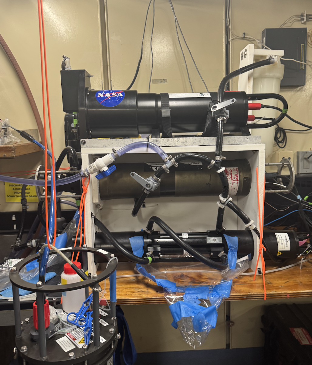
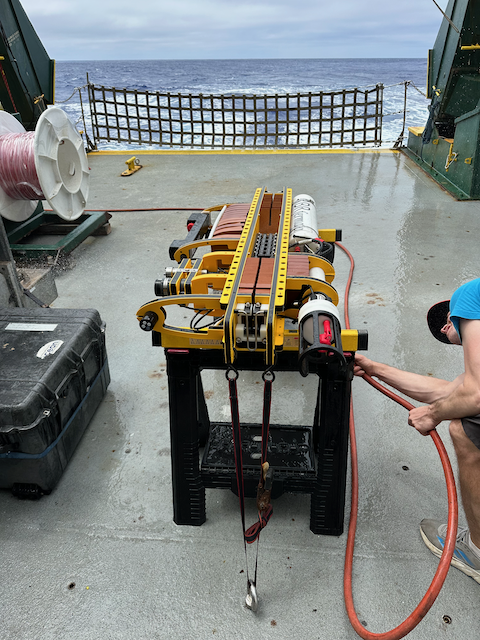
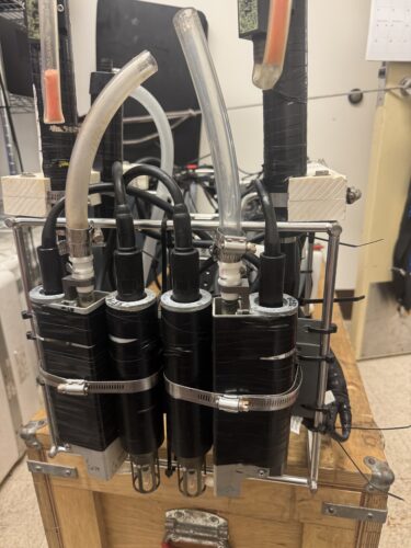
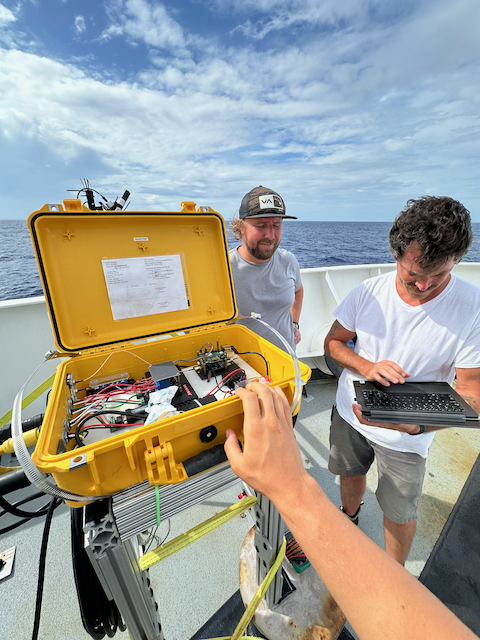
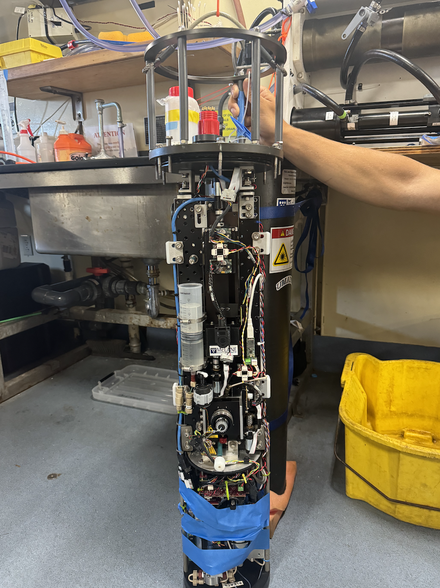– IFCB outside of its Titanium Case

This week, I also got to learn more in depth about the imaging flow cytobot instrument (IFCB). An imaging flow cytobot is used for multiple things but it can detect, size and image cells floating in the water. It’s a great tool to get an idea of community distribution of phytoplankton in real time. Most labs have a program they run the samples through that also help identify the species of phytoplankton.

However, there’s genuinely no better way to learn more about an instrument than when you’re learning to troubleshoot it to diagnose a problem. Due to the humid nature of the ship, we suspected that the humidity may have interfered with some of the sensors on the instrument. Therefore, we spent a couple of hours investigating until it was finally decided to just call the manufacturer and have them walk us through the different parts of the instruments and its troubleshooting.

Ali’s set up also features Spectral Absorption and Attenuation Sensor (AC-S), Submersible Particle Size Analyzer (LISST) and the Hyper-Spectral Backscatter Instrument (HYPER BB) all linked up to the ship’s underway system to take a look at the different properties of the water. It is super cool to say the least and I look forward to diving into more about it next week.

Cheers,

Briana

– Ferry Terminal in Mo’orea, French Polynesia

– The beautiful RV/Kilo Moana in Papeete, French Polynesia

L3W8: Swells and Station 13

By Hunter Adams

On November 26, 2024

In MATE Blog Archive, R/V Kilo Moana, University of Hawaiʻi at Mānoa, SOEST

Howdy all,

What an awesome journey we’ve had over these past two months of leg three! We’ve hit some major milestones over the last two weeks – completing all our long station sampling, wrapping up our uCTD casts, finishing the underway system collections, and getting the ship clean and packed up. Our next stop is Papeete, Tahiti, where we’ll resupply and exchange our crew and team of scientists!

Long Station 12 went off without a hitch with more successful deployents and recoveries of our CTDs and arrays. But Station 13 (appropriately named) threw us some curveballs. Our intended location for Station 13 was at 30° S location, but severe weather forced us to pivot to 27.5° S. Even there, we faced some of the roughest seas of our entire cruise. With high winds and large swells, deployments were more challenging and stressful for our equipment. Particularly pushing our CTD/rosette’s .322 electro-mechanical wire close to its safety limits.

Despite the challenges, Station 13 proved to be a triumphant finale to our main research operations. We successfully:

Deployed all ARGO and NKE floats
Secured all arrays
Collected, processed, and stored valuable hydrographic and biogeochemical data sets
Completed our 161st (and final!) celebratory uCTD cast

One of the most rewarding aspects of the SPOC cruise has been getting hands-on with our the various types of equipment. There was something special about not just operating but truly understanding and maintaining instruments like the LISST, UVP, uCTD, HyperPro, wirewalker, and various GPS beacons to name just a few. Developing this understanding has improved my confidence when working with this equipment and my technical abilities as a whole.

We’re now transitioning into the final phase of my third leg- KM2419, an ocean floor mapping cruise from Tahiti back to Hawaii. The labs are cleaned and packed, ready for the transit home and subsequent HOT cruise. Stay tuned for updates for my experiences in Tahiti and the start of the mapping cruise!

All the best,

Hunter

– Sunset from Station 12

– The birthday cake that the galley crew was kind enough to put together for me

– One of the last uCTD recoveries near 30 degrees South complete with high winds and large waves

– Briana and I post uCTD #161 recovery

– The Wirewalker stripped down for cleaning before we packed it up

– A team of awesome people celebrating the conclusion of the SPOC cruise!

End of Cruise: CTD Wrapped (Week #7, Briana Prado)

By Briana Prado

On November 25, 2024

In MATE Blog Archive, R/V Kilo Moana, University of Hawaiʻi at Mānoa, SOEST

End of Cruise: CTD Wrapped (11/17 – 11/24)

A significant portion of the work fellow MATE Intern Hunter and I did consisted of taking Conductivity, Temperature and Depth Profiles (CTD) work in two main forms; underway CTDs and CTD Rosette Cast. Over the course of this 34 day cruise, Hunter and I completed over 161 underway CTD and over 101 CTD Rosette cast, generating a nearly complete data set of a transect from 21N^o to 27 S^o.

Our 161 underway CTD cast also appears to break a couple of records by a long shot. The second, third and fourth data sets contain an already impressive 83, 48 and 45 uCTD’s, but we doubled it!

Our mentor, Tully Rohrer praised us in casting over 161 underway CTD and experiencing very minimal problems besides some mechanical issues that came with wear and tear of the instrument. Tully once painful recalled how there was a cruise where the team kept getting tangled or as Tully calls them “Wuzzles” and how long and hard it was to untangle the line for hours. Thankfully we didn’t run into any issues with that, phew!

– Tully Rohrer rinsing the underway CTD to start packing it up at the end of the cruise

I really enjoyed casting the uCTD’s because it gave us an excuse to go out and stare at the ocean every 2 hours for about 25 minutes. I was being silly one night and calculated that over the 161 cast that we completed that we both stared at the ocean for a cumulative of over 60 hours or about 30 hours each! Pretty crazy if you ask me, but super fun!

– Fellow Mate-Intern Hunter Adams and I celebrating our last uCTD

The SPOC team celebrated our last uCTD cast #161 by standing by as Hunter and I tearfully casted our last one. Data wizard Dr. Daniel Murratore promised us to analyze our cast once it was retrieved and they delivered these beautiful graphs! I am so excited to see the paper and the research that will eventually reference this impressive data set, hopefully soon!

– SPOC Team helping us celebrate our last underway CTD thus concluding a 161 run!

==========================================================

Another major and significant component of our work was the CTD Rosette Cast that took place every 3 hours while at the long stations.

There were 5 long stations, each containing about 19 – 21 CTD casts, culminating in a total of 101 CTD casts! Most cast traveled to 250 meters ~ (820 ft) since the team was mostly interested in surface processes but we did have at least two 1000 meters cast for each long stratton (for diel studies) and a handful of cast that went down to ~3500 meters for calibration purposes.

Running the CTD console was an exciting experience that taught me a bit about double checking your work, keeping cool under pressure, reading water column profiles on the fly and communicating via radio. Running the CTD was a multi step process that typically involved empty niskins, and then caulking them i.e attaching lanyards to the hooks on the CTD Rosette. Once those are attached, you turn to the bottom of the niskin where you attach the lanyard hooks to the bottom of the bottle, opening them in the process. Once the niskins are set up, you take multiple laps around the CTD, making sure that the bottle caps at the top of the nisking which control the pressure at which water leaves the spigot are closed tightly enough. Then you take another lap making sure that all the spigots at the bottom of the nisking are sticking out, so as not to lose samples when you’re moving the CTD back onto the ship. Failure to do all the steps above could result in damage to the rosette or the niskins which should be avoided at all cost.

– Briana Prado caulking CTD bottles

The last lap you take is to take off the caps off the sensors. This CTD rosette was equipped with a UVP, PAR, LIST and syringes on the oxygen sensors, so I’d have to make sure that those were off and ready to collect data. Once the CTD Rosette is set up, I turn back to the lab, collect my cast sheet and relay the information on the cast sheet to the log sheet where I’d take note of starting and ending latitude and longitude, depth of the water column, time the CTD Rosette went in and out of the water, and the depths at which we are firing the bottles. While that is happening, the Ocean Technology Group (OTG) is communicating with the Hawboldt Winch operators about picking up the slack in the wire to get the CTD ready for deployment. Once the slack has tightened, I get ready to turn on the Seabird Deck Box and to start recording on the Seasave software, a software that relays all the live information from the CTD Sensors and rosette back to the ship and the computer you’re working from. Once all that is set up and running, you communicate with the back deck and tell them the package is ready for deployment. The OTG group then checks in with the bridge to get their approval, once warranted, the OTG group checks in with the winch operators to then deploy the package.

Intern: “Back Deck – Lab, the package is ready for deployment.”

OTG: “Roger that lab, Bridge-Back Deck “Can we deploy this package?”

Bridge: “Back Deck- Bridge, You are clear to deploy the package.”

OTG: “Roger that, Winch-Back Deck, Are we clear to deploy the package?

Winch Operators: “Back Deck-Winch, Roger, We are now deploying the package”

Once in the water, we let the CTD soak at the surface, to allow the sensors to equilibrate with the water temperature and start pumping water through the sensors. After about a minute, I radioed the Back Deck to take the CTD to a pressure-depth of 15 deci-bars at 30 meters per minute. It is essential that the package travel at this specific speed as that is how the CTD sensors are turned on.. Once the CTD pumps are on, I communicate again with a back deck OTG person that we are now clear to take the package back to the surface and then to Target depth ~ 250 meters. Once that is done, we are now ready to take our water column profile.

The CTD profile generates right in front of your eyes. It’s always fun to take note of the chlorophyll maximum or the part of the water column, where most of the phytoplankton are hanging out and see how that changes, hour to hour, based on the time of the day, where we are in the ocean and other oceanographic parameters like oligotrophic waters. Other things we keep an eye out for is the Cpmax or the area of the water column with the highest concentration of particles.

Once we reach our desired depth of lets say ~250 m, we are clear to start firing bottles. The winch operator will declare they have reached the desired pressure/depth.

Winch: “Lab-winch we’ve have hit target depth 250 db or 2-5-0 decibars”

Intern: “Winch- lab, next target depth is 125 db or 1-2-5 decibars”
Winch: “Roger that “Next target depth is 125 or 1-2-5 decibars”

We then wait for the winch to call out 125 decibars, which we double confirm by looking at the screen and reading where the CTD tells us it is in the water column. Once we’ve reached the desired depth, I wait 30 seconds to fire the first bottle. This time is allotted to allow for any disturbances in the water column to settle. Once I fire the first bottle any subsequent bottles are fired at 10 second intervals, for the same reason.

Once I’ve fired the bottles I call out to the winch our next target depth and repeat.

Once we’re near the surface, I call out to the back deck and tell them that we are now clear to recover the package and OTG begins checking in with the winch and bridge folk to confirm they are also ready to recover.

Once the package is recovered, I finish jotting down the meteorological data, log the event in the event page and turn off the deck box. It is paramount to turn off the deck box because you don’t want to electrocute anybody when they start releasing the slack on the wire.

For our last cast, cast #101, we went down to a depth of 3500 meters (~11,480 ft). This cast was used to calibrate the CTD’s oxygen sensors and also collected water from the Antarctic Deep Water water mass. As the name implies, this is water that last saw the surface of the ocean, when it downwelled off the coast of Antarctica. As a result the water is super cold, oxygen rich and salty! Chief Scientist Angelicque White was super cool and boiled down the water to collect and bottle salts for us as a memoir as well as let us cast away a couple pieces of styrofoam to crush them underpressure. We didn’t have too much styrofoam so we had to experiment with different types… some were more succesful than others.

– Before and after pictures of our styrofoam squares that went down to a depth of 3500 meters!

Now that we are done with all the stations, we’ve started to pack up labs. We will be arriving to Tahiti soon, stay tuned!

Cheers,

Briana